Background

A while ago, a fellow member of the Fr334aks team asked me to take a look into a now retired Hack The Box challenge which involved breaking the Bifid cipher to recover a flag. I was unable to solve this challenge at first (which was quite frustrating), but a few days later I found this post showcasing a way to break this kind of cipher using a Simulated Annealing algorithm, a technique also used to break the Playfair cipher.

I wasn’t familiarized with this algorithm but after some reading, I found it to be somewhat similar to another class of metaheuristic search commonly employed for optimization problems: Genetic Algorithms. As I was still frustrated by not being able to solve the challenge in the first place and also needed to work out something as the final project for my Artificial Intelligence class, I decided to join the two things and use and develop a Genetic Algorithm that could break the Bifid Cipher.

Using GA as a means to perform cryptanalys is not at all a new idea and there are a lot of papers on this topic already. Based on a few of these, I wrote a simple code to solve the challenge and then performed some tests, with different text sizes and parameters. The results were presented in the form of a short paper to my AI class.

The resulting algorithm succeeded in recovering the contents of a ciphertext from which the writing language is known, as long as the ciphertext sample has a sufficient length. In particular, small ciphertext samples (less than 200 letters) are quite hard to recover completely and multiple tries might be necessary.

In this post I will go through the workings of the Bifid cipher as well as the concept and design of a Genetic Algorithm that can be used to break it.

The Bifid cipher

The Bifid cipher was created by the french cryptographer Felix Delastelle around 1901 (the year might diverge depending on the source) and apparently was never used for any serious purpose, even though it was quite hard to break it at the time and yet very simple to use, what made it very popular with amateur criptographers.

The cipher combines substitution and transposition, what makes it stronger than a regular substitution cipher. The substitution is performed using a Polybius square, a 5x5 square where each position is occupied by a letter of the alphabet (letters I and J are considered the same symbol), like in the following example:

	0	1	2	3	4
0	X	I	P	R	H
1	Y	Q	K	A	T
2	D	S	F	L	N
3	O	B	E	M	V
4	C	G	Z	U	W

The key is a permutation of the alphabet that is written within this square, forming what is called a key-table or key-square.

To encrypt a message, first we choose an integer value b (b > 1) called period or block size. The message is then broken into various blocks of this size, padded with random letters if necessary, and each block is enciphered separately using the following procedure:

Lookup the position of each letter of the block at the key-table.
Write down the row index of each letter in a line
Write down the column index of each letter in another line
Join these two lines by appending the second at the end of the first
Form new coordinates by reading these values in pairs
Lookup the resulting ciphertext at the key-table

For example, let’s encrypt the word “PASSWORD” using the previous key-square and just for the sake of demonstration, consider b=8. First we find the position of each letter.

	P	A	S	S	W	O	R	D
Row	0	1	2	2	4	3	0	2
Column	2	3	1	1	4	0	3	0

Now we append the column indexes at the end of the row’s

0 1 2 2 4 3 0 2 2 3 1 1 4 0 3 0

And reading these values in pairs, we get:

(0, 1) = I
(2, 2) = F
(4, 3) = U
...

So the word “PASSWORD” becomes “IFUPLQCO”. To decrypt it, we would do the same process in reverse:

Lookup the position of each letter of the block at the key-table.
Write down the row and column indexes of each letter in the same line
Split this line in the middle, creating another line below it
Form new coordinates by reading each column
Lookup the resulting plaintext at the key-table

To reverse “IFUPLQCO”, we would first do

 I   F   U   P   L   Q   C   O
0 1 2 2 4 3 0 2 2 3 1 1 4 0 3 0 

And then split it in two

 0  1  2  2  4  3  0  2 
 2  3  1  1  4  0  3  0 

Now we read each column as a pair of coordinates on the key-table:

(0, 2) = P
(1, 3) = A
(2, 1) = S
...

And we get “PASSWORD” back. Note that in this scheme, all letters are uppercase and any other symbol is removed.

As the key is a permutation of the alphabet, there are 25! (or around \(1.5 * 10 ^ {25}\)) possible keys, which is a huge number. However, the number of distinct blocks for a fixed period is generally way smaller, so there should be multiple keys that produce the same text [1].

As you might have noticed, to attack this cipher first we need to find the block size, or it might not be possible to recover the text even with the right key. Finding this value can be trivial if the blocks are clearly separated by some character as it is sometimes the case, but we can’t always count on it, so we need a consistent method to figure b.

In his work, [1] defines an efficient method to determine b from the ciphertext by counting the frequency of pairs of letters that appear repeated at regular intervals of size d and then plotting the results in a graph as a function of d, resulting in a periodic function whose period is equal to the block size. A simplified version of this method is presented by [2]. For the remaining of this post, let’s assume that the block size is known.

Genetic Algorithm

Now that we know how the Bifid cipher works, we can talk about the technique used to break it. Let’s start with some theory

What is a Genetic Algorithm?

As per Wikipedia, “In computer science and operations research, a genetic algorithm (GA) is a metaheuristic inspired by the process of natural selection that belongs to the larger class of evolutionary algorithms (EA)”.

In short, a GA is a general optimization algorithm that works by mimicking the process of biological evolution, by applying the principle of Natural Selection, where only the best individuals of a population survive and reproduce, resulting in better adapted individuals over time.

Bringing this into a computational context, that means that we will improve the solutions to a problem over a number of iterations, and our solutions should get better every time until an optimal point is reached. That doesn’t necessarily means the best solution (global optimum), but a good enough solution to our problem (local optimum).

Ok, but how does it work, exactly?

There are various ways to design a GA, but in general we start with an initial population of randomly generated individuals called cromossomes, each of which represents a possible solution to the problem we are attacking.

Then, the evolution process is performed through a number of generations. At each generation, there are multiple rounds where two or more parents are choosen from the current population to reproduce in what is called a crossover operation, resulting in an offspring which is a combination of its parents’ features.

Sometimes, this offspring can go through a mutation process, introducing genetic variability to evolve traits that aren’t present in any of it’s parents. And after that, this new individual can be integrated into the population and the process continues.

Both the crossover and mutation operations are stochastic events, whose probability of ocurring can be adjusted by changing the parameters of the algorithm, what makes it very adaptable.

This stochastic behaviour might sound weird at first, as it seems that what we are doing is just a random search, however this is exactly what makes the algorithm work. A GA is what is called a metaheuristic – a fancy way of saying that they search for an aproximate solution to a specific problem, by progressing in a directed fashion through the search space, comprised by the universe of possible solutions, narrowing down the possibilities by climbing towards the better looking solutions until one is found that met some predefined criteria to be considered optimal.

The key to a GA effectiveness is how we apply the Natural Selection principle to the evolution process, after all our goal is to get a better solution at each generation. There are many different strategies to ensure the population is improving, but the most common way to do this is by discarding the worst individuals of each generation, only allowing the best solutions to evolve further.

To do that, we need to define a function to score each solution, allowing us to measure how good they are in comparison to each other. Such function is usually called a fitness or objective function and is specific of each problem.

Defining the fitness function is a crucial step of a GA’s design and has a huge influence in its performance and capacity to solve the problem. We will talk about how to define this function later, but for now it is enough to say that we need a way of scoring the cromossomes.

The algorithm starts with random values and evolves by combining different individuals and keeping only the best traits, trying get at least close to a better solution every time. However, just like with biological evolution, there are some limitations to this process. One such limitation is related to how the search is performed.

Since we can’t ensure that our initial population has the traits necessary to solve the problem, there is no guarantee that they will ever evolve into a valid solution. Worse than that, the combination of traits that form a solution in the search space can be very complex, so it might be the case that by selecting only the best individuals of the current population, we will end up losing some specific trait that would result in a better solution many generations later. This way, the algorithm will converge to a suboptimal solution and stop improving.

For example, consider the case in which we try to find the maximum point of a function f(x) whose domain is shown in the graph below:

Function1

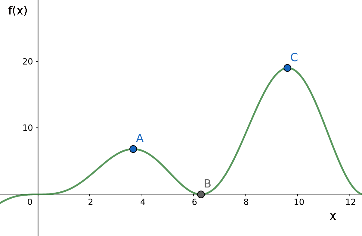
Now, suppose that currently our best solution is located in point A and the algorithm evolves by moving along the X axis. In this case, even though point C is clearly the maximum of this function, we won’t be able to reach it, as it would be necessary to pass through point B which is a worst solution than the one we currently have. A GA is an oportunistic algorithm and will only follow a path if it clearly leads to a better solution in a short term.

And here the inherent randomness of the evolution process plays an important role in avoiding such a scenario, as it can help us escape this local optimum possibly aproximating the global maximum.

That is the purpose of the mutation operations. If we mutate some of the new individuals at each generation in a random way (throwing them along the X axis), maybe (just maybe) they would reach the point C or some other point between B and C with a higher image than A and then continue evolving from there.

“Ok, but when do we stop?” Well, whenever you want. Just set a condition on your code to stop evolving at some point. For example, when the best individual of the population doesn’t change for a specific number of generations, or when the mean deviation of all cromossomes is below a certain threshold, or whatever. Its up to you to decide and this could take some trial and error to figure out, just like most things when dealing with such evolutionary algorithms.

Designing a GA to break the Bifid cipher

Now that we talked about the theory behind it, let’s design our own algorithm to break Bifid. First, we need to decide how we are going to encode our solutions as cromossomes. To do that, first we need to know what exactly would be a solution to such problem and what we are actually searching for.

If our goal is to reveal a text that was enciphered using a key, we can resume the problem to finding one such key that will allow us to perform the reverse process. In the case of Bifid, the keys are just permutations of the alphabet and that is what our cromossomes should represent. As such, the cromossomes could consist of an array of 25 distinct letters of the alphabet in any order (remember that J and I are considered the same symbol).

The next step is defining the fitness function that will be used to score each cromossome. This function should take a cromossome as input and output a numerical value representing its quality as a solution. Again, we must consider the specifics of the problem in order to choose an effective function to evaluate the solutions.

The insecurity of most classical ciphers is often attributed to their simplicity and susceptibility to exploitation by advances in cryptanalysis techniques. It’s important to recognize that classical ciphers were not originally designed with the principles of confusion and diffusion in mind. Confusion involves creating a complex and nonlinear relationship between the ciphertext and the key, making it challenging for attackers to derive the key from the ciphertext. Meanwhile, diffusion aims to ensure that changes in the plaintext are thoroughly distributed throughout the ciphertext and vice versa, enhancing overall security.

The presence of multiple keys producing the same ciphertext/plaintext pair in the Bifid cipher is a big problem. However, the most significant issue lies in the fact that an incorrect key can still produce a partially readable text, as long as a sufficient portion of the key characters is correct. This particular weakness is what we are going to use for scoring the chromosomes.

If we use each cromossome’s key to decrypt the ciphertext and analyze how much of it becomes readable, we can measure how close it is to the correct solution. Measuring how much a sequence of characters looks like valid text is a common problem in Cryptology, usually addressed using techniques like frequency analysis. This method involves counting the ocurrences of certain patterns composed by sequences of adjacent symbols observed in an written language and comparing to the known frequency for that language.

There are various techniques available to validate if a given text corresponds to a particular language. One commonly employed method is Friedman’s Most-Frequent-Letters test, often referred to as the MFL score. This test involves calculating cumulative frequencies of each character in the text relative to the language in which it is assumed to be written. Formally, given a sequence of n characters represented as α = {L₀, L₁, …, Lₙ₋₁}, the MFL score is computed as follows:

\[MLF(\alpha) = \sum\limits_{i=0}^{n-1} freq(L_{i})\]

Where \(freq(L_{i})\) denotes the (normalized) frequency in which the character L appears in a specific language. For example, if the plaintext was written in english and we have a candidate string of “HELLO”, its MFL score would be a sum of the frequencies of each these letters in the english language like:

MFL(HELLO) = freq(H) + freq(E) + freq(L) + freq(L) + freq(O)

If we consider the frequencies given here, this score would be:

MFL(HELLO) = 5.05 + 12.49 + 4.07 + 4.07 + 7.64 = 33.32

It is a simple but also very effective technique. The problem is that sometimes (specially for shorter texts) it might result in misleading scores. For example, in the english language the sequence “EEEEEEEEEE” has an higher score than any other sample of the same length even though it is clearly not a valid text.

There are many other techniques that could be used to archieve the same goal, with varying degrees of success. If you are interested here you can learn about a few other methods, as well as some mathematical background for statistical properties of languages.

In my approach, I’ve opted for a variation of the MFL score that centers around the cumulative frequency of bigrams, which are sequences of two adjacent symbols, as opposed to individual letters. While there isn’t a specific reason behind this choice, and there may be alternative methods available, I found that this variation performed well in my tests.

Having defined the cromossomes and how to score them, we need to define three important operations:

Selection - how to select cromossomes as parents
Crossover - how the parents will reproduce
Mutation - how the offspring will be mutated

For the selection I used a common method called Fitness Proportionate, sometimes refered to as “roulette wheel”. This method works by calculating the sum of the fitness of each cromossome and giving it a chance to be selected that is proportional to the cromossome fitness over the sum [3]. If we have N cromossomes \(C_{0}\) to \(C_{N-1}\) with fitness \(F_0\) to \(F_{N-1}\), the chance of the cromossome \(C_j\) being selected can be expressed as

\[P(C_j) = \frac{F_j}{\sum\limits_{i=0}^{N-1} {F_i}}\]

We can then use these values to generate biased random numbers, i.e random numbers following a distribution in which each of them have different probabilities of appearing (more on that later). This way, the best individuals will have more chances of being selected for reproduction than the others.

And speaking about reproduction, we also need to decide how they are going to do this. As the resulting offspring should contain caracteristics of both parents, the obvious answer is to create a new cromossome that has half the of the symbols of each parent. However, keep in mind that our cromossomes represent keys composed of 25 different letters and we must ensure that this property will hold in the offspring.

My implementation of this operation was to choose a random crossover point between 1 and 25, then copy from the first parent all the characters up until that point and the remaining characters would come from the second parent, but the letters already copied from the first would be ignored.

For the mutation we could use any random change in the offspring that doesn’t depend on the parents. For example, swapping two letters at random positions.

Now we have almost everything we need and can start to think on how it is going to work. As I’ve mentioned before, the algorithm will take a few parameters that influence its behaviour, allowing us to adjust it if necessary. These parameters are:

Crossover rate: Likehood of producing an offspring
Mutation rate: Likehood of mutating an offspring
Population size: The initial size of the population
Number of generations: Maximum number of generations
Crossover rounds: Maximum crossovers per generation

The chosen parameters were:

Crossover rate = 0.8 (80% chances of reproduction)
Mutation rate = 0.6 (60% chances of mutation)
Population size = 4000
Number of generations = 12000
Crossover rounds = 1400

It is worth to mention that there is “no one size fits all” and the parameters mentioned earlier were selected after several iterations and experiments. However, they are not guaranteed to be the best for every problem. Depending on the specific problem, its characteristics, and the behavior of the genetic algorithm, fine-tuning and adjustment of these parameters may be necessary to achieve the best results.

To sum it up

We start with a population of randomly generated individuals consisting of permutations of the alphabet and will iterate over a number of generations.

At each generation, a specified number of crossover rounds will be performed. During each of these rounds, a random number in the range of 0 to 1 will be generated. If this number falls below the predefined crossover rate, a crossover operation will occur.

The selection of parents for the crossover operation will be determined using the roulette wheel selection. This mechanism assigns a probability of selection to each individual in the population based on their fitness. Individuals with higher fitness scores will have a greater chance of being selected as parents for the crossover.

Once the parents are chosen, the crossover operation will combine genetic material from two parents to produce one or more offspring. The chosen crossover method works by selecting a random crossover point and ensuring that genetic material from the first parent up to that point is included in the offspring, while the remaining genetic material comes from the second parent, with duplicates from the first parent being ignored.

This new individual may undergo a mutation process depending on another random number generated within the range of 0 to 1. This mutation operation involves swapping the positions of two symbols within the alphabet at random.

After the crossover operation, the algorithm will assess the quality of the resulting offspring and will add it to the current population only if it demonstrates better fitness (i.e., a higher fitness score) than the worst-performing individual currently present in the population.

The worst cromossomes will be eliminated to keep the same population size after each generation. This step ensures that the overall quality of the population improves over time. New, potentially superior individuals are introduced, replacing the weakest members of the population. This dynamic process encourages the population to evolve towards better solutions, bringing the decrypted text ever closer to the original plaintext ~~(or at least that is what we hope for)~~.

This process of selection, crossover, and potentially mutation will be repeated for a specified number of generations. Additionally, our algorithm includes a stopping condition that triggers when a maximum number of generations without fitness improvement is reached.

Results

To validate the algorithm, I perfomed a series of tests using different texts (both English and in Portuguese) with sizes varying from 200 to 500 characters, ciphered with a random key-table. For each text length, I ran the algorithm until I got the correct plaintext 3 times, even though a partially decrypted text could still be read with some effort.

Since I knew the original text, I also added a condition to stop as soon as it was fully recovered, so I would know exactly how many generations it took. The results for the texts in English are presented below:

Text Size	Attempts	GR 1	GR 2	GR 3	Average
203	11	1365	1884	3815	2355
302	7	2102	1321	1710	1711
404	6	1290	1366	1623	1426
499	3	509	631	497	547

And the results for Portuguese texts:

Text Size	Attempts	GR 1	GR 2	GR 3	Average
206	14	1807	748	2394	1650
305	9	1309	865	1738	1304
400	9	1698	711	1645	1351
497	4	402	446	710	520

In both these tables, “GR X” means the number of generations needed to recover the plaintext for the Xth time.

Based on the results, we can see that the number of generations required to successfully decrypt the cipher is inversely proportional to the size of the ciphertext. In other words, as the ciphertext sample becomes smaller, the task of recovering the plaintext becomes increasingly harder.

I also conducted experiments with smaller texts, approximately 100 characters in length. These smaller ciphertexts proved to be considerably more challenging to recover, often requiring numerous attempts. In fact, out of 15 attempts, I successfully recovered the plaintext once.

You can access the algorithm by following this link: GitHub - ga-breaking-bifid. While I acknowledge that this algorithm may not be considered optimal, I found the process of creating it to be quite fun.

If you’re interested in delving deeper into Genetic Algorithms, I highly recommend the excellent book titled ‘An Introduction to Genetic Algorithms’ by Melanie Mitchell. You can find it here.

I hope my explanation has been clear, although I must admit that I might not be the most didactic communicator. This book, however, provides a comprehensive and structured introduction to the fascinating field of Genetic Algorithms, offering a solid foundation for further exploration.

Thank you all for reading. See you next time.